Signal Separation in Electron Microscopy

Oftentimes in an X-ray energy dispersive spectroscopy (EDS) analysis, the desired result is a quick understanding of what phases are present within a dataset rather than an exact quantitative elemental characterization. A clear picture of what elements are spatially correlated and where they are located is often enough to answer the research question at hand. Commercial EDS vendors have realized this, and almost every available software package includes some option of “phase mapping” (e.g. Oxford – AutoPhaseMap, EDAX - Smart Phase Mapping, Bruker – AutoPhase, etc.). Most operate as some proprietary form of principal component analysis (PCA), and are often “black box” in nature, with no indication of what algorithm was used or how the results were obtained. This presents a significant challenge for comparisons between different vendors’ systems and hinders efforts towards more open and reproducible science.

Thankfully, EDS mapping is not unique in terms of the need to identify “pure phases” within hyperspectral data; the fields of remote sensing and chemometrics have been developing factor analysis tools for this problem since the 1970s¹, and many of the methods used in those disciplines can be directly applied to EDS data with only minor changes to their implementation. In fact, the first examples of EDS factor analysis were reported over 20 years ago², but the methods have seen only limited use since that time, due in part to “lock-in” from vendor software and the lack of easy to use tools. Considering this, the recent development of open-source software tools for hyperspectral data analysis that can read the data output by proprietary vendor software packages (e.g. HyperSpy³) has made it relatively simple to perform advanced EDS analysis beyond the scope of the vendor software packages.

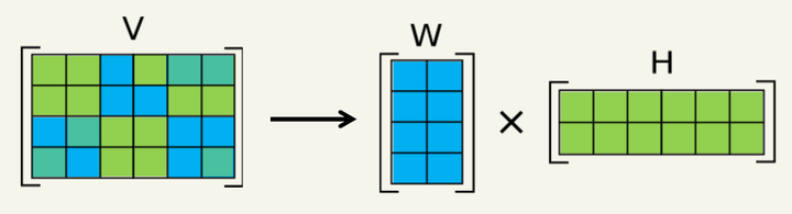
In an EDS spectrum image, each spatial position contains a spectrum that is a mixture of signals from one or more “prototype” spectra or “pure phases.” The goal of hyperspectral unmixing is to accurately determine those spectral prototypes (called components or endmembers) and the strength or weight of each component at each pixel (called a loading or score map). This is an unsupervised machine learning problem of factor analysis, where the computer code should identify and describe the interesting components, without input from the user. There are many algorithms available to perform this task, each with associated benefits and drawbacks depending on the assumptions made by the algorithm.

In our work, we investigate numerous methods of spectral unmixing performed on both simulated and experimental EDS spectrum images to compare their performances. Among the algorithms examined are: PCA + independent component analysis (ICA)⁴, non-negative matrix factorization (NMF)^{5 6}, multivariate curve resolution (MCR)¹, vertex component analysis (VCA)⁷, Bayesian linear unmixing (BLU)⁸, and simplex identification via split augmented Lagrangian (SISAL)⁹.